
My article, Replicating Group-Based Trajectory Models of Crime at Micro-Places in Albany, NY was recently published online first at the Journal of Quantitative Criminology (here is a pre-print version, and you can get my JQC offprint for the next few weeks).
Part of the reason I blog is to show how to replicate some of my work. I have previously shown how to generate the group based trajectory models (1,2), and here I will illustrate how to replicate some of the point pattern analysis I conducted in that paper.
A regular task for an analyst is to evaluate spatial clustering. A technique I use in that article is to use Ripley’s K statistic to evaluate clustering between different types of events, or what spatial statistics jargon calls a marked point pattern. I figured I would illustrate how to do this on some example point patterns of shootings, so analysts could replicate for other situations. The way crime data is collected and geocoded makes generating the correct reference distributions for the tests different than if the points could occur anywhere in the study region.
An example I am going to apply are shooting incidents that have marks of whether they hit the intended victim or missed. One theory in criminology is that murder is simply the extension of general violence — with the difference in aggravated assault versus murder often being happenstance. One instance this appears to be the case from my observations are shootings. It seems pure luck whether an individual gets hit or the bullets miss everyone. Here I will see if there appear to be any spatial patterning in shots fired with a victim hit. That is, we know that shootings themselves are clustered, but within those clusters of shootings are the locations of hits-and-misses further clustered or are they random?
A hypothetical process in which clustering of shooting hits can occur is if some shootings are meant to simply scare individuals vs. being targeted at people on the street. It could also occur if there are different tactics, like drive-bys vs. being on foot. This could occur if say one area had many shootings related to drug deals gone wrong, vs. another area that had gang retaliation drive by shootings. If they are non-random, the police may consider different interventions in different places – probably focusing on locations where people are more likely to be injured from the shooting. If they are random though, there is nothing special about analyzing shootings with a person hit versus shootings that missed everyone – you might as well analyze and develop strategy for all shootings.
So to start we will be using the R statistical package and the spatstat library. To follow along I made a set of fake shooting data in a csv file. So first load up R, I then change the working directory to where my csv file is located, then I read in the csv into an R data frame.
library(spatstat)

#change R directory to where your file is
MyDir <- "C:\\Users\\andrew.wheeler\\Dropbox\\Documents\\BLOG\\R_shootingVic\\R_Code"
setwd(MyDir)

#read in shooting data
ShootData <- read.csv("Fake_ShootingData.csv", header = TRUE)
head(ShootData)
The file subsequently has four fields, ID, X & Y coordinates, and a Vic column with 0’s and 1’s. Next to conduct the spatial analysis we are going to convert this data into an object that the spatstat library can work with. To do that we need to create a study window. Typically you would have the outline of the city, but for this analysis the window won’t matter, so here I make a window that is just slightly larger than the bounding box of the data.
#create ppp file, window does not matter for permuation test
StudyWin <- owin(xrange=c(min(ShootData$X)-0.01,max(ShootData$X)+0.01),yrange=c(min(ShootData$Y)-0.01,max(ShootData$Y)+0.01))
Shoot_ppp <- ppp(ShootData$X, ShootData$Y, window=StudyWin, marks=as.factor(ShootData$Vic), unitname = c("meter","meters"))
Traditionally when Ripley’s K was originally developed it was for points that could occur anywhere in the study region, such as the location of different tree species. Crimes are a bit different though, in that there are some areas in any city that a crime basically cannot occur (such as the middle of a lake). Also, crimes are often simply geocoded according to addresses and intersections, so this further reduces the locations where the points can be located in a crime dataset. To calculate the sample statistic for Ripley’s K one does not need to account for this, but to tell whether those patterns are random one needs to simulate the point pattern under a realistic null hypothesis. There are different ways to do the simulation, but here the simulation keeps the shooting locations fixed, but randomly assigns a shooting to be either a victim or a not with the same marginal frequencies. That is, it basically just shuffles which events are counted as a victim being hit or one in which there were no people hit. The Dixon article calls this the random relabelling approach.
Most of the spatstat functions can take a separate list of point patterns to use to simulate error bounds for different functions, so this function takes the initial point pattern, generates the permutations, and stuffs them in a list. I set the seed so the analysis can be reproduced exactly.
#generate the simulation envelopes to use in the Cross function
MarkedPerms <- function(ppp, nlist) {
  require(spatstat)
  myppp_list <- c() #make empty list
  for (i in 1:nlist) {
    current_ppp <-  ppp(ppp$x, ppp$y,window=ppp$window,marks=sample(ppp$marks))  #making permutation
    myppp_list[[i]] <- current_ppp                                               #appending perm to list
  }
  return(myppp_list)
}

#now making a set of simulated permutations
set.seed(10) #setting seed for reproducibility
MySimEvel <- MarkedPerms(ppp=Shoot_ppp,nlist=999)
Now we have all the ingredients to conduct the analysis. Here I call the cross K function and submit my set of simulated point patterns named MySimEvel. With only 100 points in the dataset it works pretty quickly, and then we can graph the Ripley’s K function. The grey bands are the simulated K statistics, and the black line is the observed statistic. We can see the observed is always within the simulated bands, so we conclude that conditional on shooting locations, there is no clustering of shootings with a victim versus those with no one hit. Not surprising, since I just simulated random data.
#Cross Ripleys K
CrossK_Shoot <- alltypes(Shoot_ppp, fun="Kcross", envelope=TRUE, simulate=MySimEvel)
plot(CrossK_Shoot$fns[[2]], main="Cross-K Shooting Victims vs. No Victims", xlab="Meters")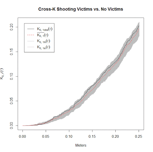
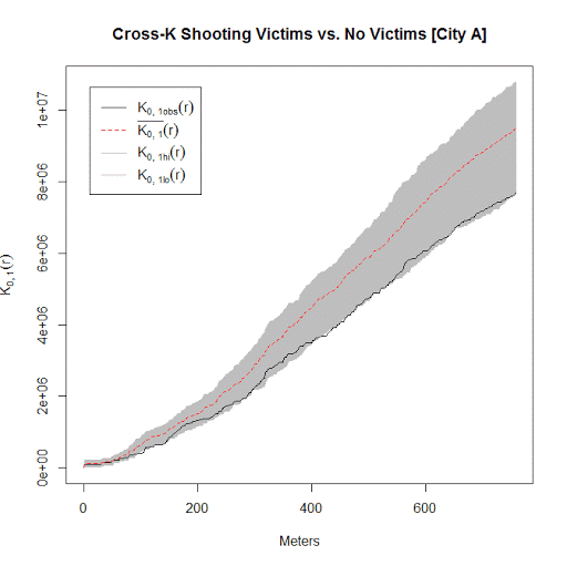
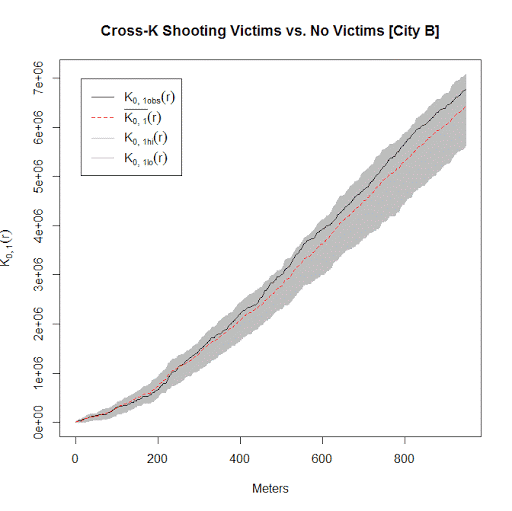
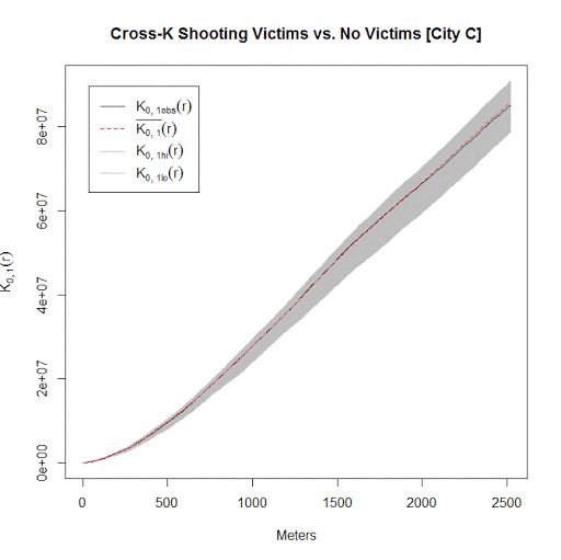
I conducted this same analysis with actual shooting data in three separate cities that I have convenient access to the data. It is a hod podge of length, but City A and City B have around 100 shootings, and City C has around 500 shootings. In City A the observed line is very near the bottom, suggesting some evidence that shootings victims may be further apart than would be expected, but for most instances is within the 99% simulation band. (I can’t think of a theoretical reason why being spread apart would occur.) City B is pretty clearly within the simulation band, and City C’s observed pattern mirrors the mean of the simulation bands almost exactly. Since City C has the largest sample, I think this is pretty good evidence that shootings with a person hit are spatially random conditional on where shootings occur.
Long story short, when conducting Ripley’s K with crime data, the default way to generate the simulation envelopes for the statistics are not appropriate given how crime data is recorded. I show here one way to account for that in generating simulation envelopes.


2 Comments