Will be a long post today, have some updates on a preprint, quotes on Flock cameras, an upcoming webinar, plus some R analysis examples of monitoring time between rare crime events.
Pre-print on JTC and examining the Buffer Zone
For a few updates on other projects, I have a pre-print out with Kim Rossmo, The Journey-to-Crime Buffer Zone: Measurement Issues and Methodological Challenges.

Two parts to this paper. Part 1, to test whether a journey to crime (JTC) distribution conforms to a buffer zone (an area with lower, but non-zero, probability of offending nearby their home for predatory crimes against strangers), it only makes sense to look at an individual offenders JTC. This is because mixtures of multiple offenders can each individually have a buffer, but in the aggregate do not (in particular if offenders have varying travel distances). This is the same point in Van Koppen & De Keijser (1997), and the fact that offenders have different travel distance distributions is pretty well established now (Andresen et al., 2014, Drawve et al., 2015; Townsley & Sidebottom, 2010).
The second part is given we need to examine individual offenders, I worked out estimates of how many observations you need to effectively measure whether a buffer zone exists. I estimate you need around 50 observations when using a gamma distribution to measure the existence of a buffer vs monotonically decreasing. Above graphs shows a kernel density estimator that takes into account to not smear the probability below 0 distance, using a transform trick to calculate the KDE on the log scale and then back transform. Both case studies we look at suggest a more peaked distribution for the buffer than gamma probably makes more sense for those samples, but pretty strong evidence the buffer exists. The code to replicate the methods and papers findings is on Github.
If you are a department and you have a good case study of a prolific offender get in touch, would be happy to add more case studies to the paper. Part of the difficulty is having high fidelity measures, offenders tend to move a lot (Wheeler, 2012), and so it is typically necessary to have an analyst really make sure the home (or nearest anchor node) locations are all correct. In addition to most prolific offenders don’t have that many observations.
Flock Story
For a second update, I had a minor quote in Tyler Duke’s story on Flock Cameras in North Carolina, Camera by camera, North Carolina police build growing network to track vehicles. I think license plate readers are good investments for PDs (see Ozer 2016 for a good example, I actually like the mobile ones in vehicles more than fixed ones, see Wheeler & Phillips, 2018 for a case study in Buffalo using them at low friction road blocks). But I do think more regulation to prevent people doing indiscriminate searches is in order (similar to how doing background checks in most states have state rules).
I get more annoyed by Flock’s advertising that suggests they solve 10% of crime nationwide, which is absurd. It is very poorly done design (Snow & Charpentier, 2024) that does a regression of clearance rates regressed on cameras per officer, and suggests the cameras increase clearance rates by 10%. There is multiple things wrong with this – interpreting regression coefficients incorrectly (an increase in 1 in camera per-officer is quite a few cameras and does not in translate to they increase clearances 10% in toto), confounding in the design (smaller agencies with higher clearance by default will have more cameras per officer), not taking into account weights in the modeling or interpretation (e.g. a 20% increase in a small department and a 0% increase in a large department should not average to an overall 10% increase). Probably the worse part about this though is extrapolating from they have cameras in a few hundred departments to saying they help solve 10% of crime nationwide.
It is extra silly because it does not even matter – it makes close to no material difference to the quality of Flock’s products (which look to me high quality, they certainly don’t need to increase clearance rates by 10% to be worth investing in ALPRs for an agency, ALPRs are so cheap if a single camera helps with say 10-20 arrests they are worth it). If anyone from Flock is listening and wants to fund a real high quality study just let me know and ask, but this work they have put out is ridiculous.
Tyle Duke’s (and the Newsobserver in general) I think do a really good job on various data stories. So highly recommend checking out that and their other work.
Webinar on Monitoring Temporal Crime Trends
I am doing a webinar for the Carolina Crime Analysis Association on Monitoring Temporal Crime Trends at the end of the month on May 31st.

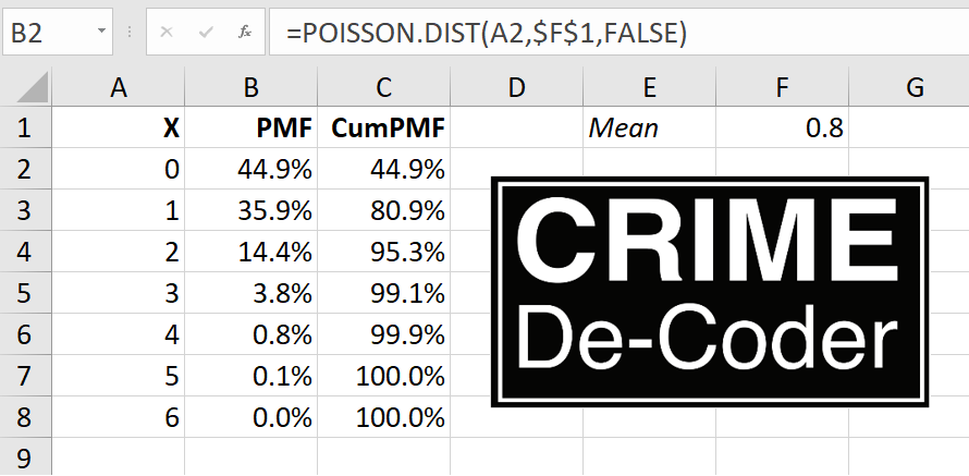
Free for CCAA members and $10 for non-members. I will be going over work I have written in various places before, such as the Poisson Z-score for CompStat reports (Wheeler, 2016). I did a recent blog post on the Crime De-Coder site on using the Poisson distribution to flag outliers for rare crime events, e.g. if you have 0.8 robberies per month, is a month with 3 robberies weird?
For other regional crime analysis groups, if you have requests like that feel free. I am thinking I want to spend more time with regional groups than worrying about the bigger IACA group going forward.
And this Poisson example segways into the final section of the blog post.
Monitoring Time in Between Events
So the above of using the Poisson distribution to say is 3 robberies in a month weird, you have to think about the nature of how a crime analyst will use and act on that information. So in that scenario, that may be an analyst has a monthly CompStat report, and it is useful to say ‘yeah 3 is high, but is consistent with chance variation that is not uncommon’. In this scenario though, if you have counts that are high, it is not the best (although better than nothing) to wait until the end of the month CompStat report.
Another common case though is the analyst is regularly reading reports, and they come in and read a new robbery, and right then and there say “I feel like there are more robberies than usual”. How would they tell then if there are more than you would expect? It does not make sense to wait for the end of the month (you technically can back-calculate in the prior month and use a scan statistic, but I think what I will suggest below is a more diagnostic approach).
Here I will outline an approach by examining the time in between events, which is motivated by a comment Rob Fornango mentioned on LinkedIn.
So there is a duality between the Poisson distribution and the exponential distribution – if you have a mean of 0.8 events per month, the inter-arrival times are exponentially distributed with a mean of 1/0.8. The typical motivation for a Poisson distribution is the inter-arrival times are independent, so you can technically just work with the inter-arrival times directly.
Here is a quick simulation in R to show that you can simulate inter-arrival times, and then turn them into counts per unit time. The counts per unit time will then be Poisson distributed. Note that R you give the lambda term directly in the R parameterization, whereas others (like in scipy) you specify 1/lambda. I know it is not documented well, but I leave as an exercise to the reader who cares enough to figure out what I am doing here and why.
set.seed(10)
pmean <- 0.8
n <- 50000

re <- rexp(n,pmean) # simulating exponential
rec <- cumsum(re)   # translating to times
frec <- floor(rec)  # will aggregate to counts per 1 unit

# factor is to include units with 0 counts
recV <- 0:max(frec)
frec <- factor(frec,levels=recV)
re_tab <- as.data.frame(table(frec))
re_tab$frec <- recV
re_tab$Freq <- factor(re_tab$Freq,levels=0:max(re_tab$Freq))

# Two tables are to aggregate to units, and then get a count
# of counts per unit
count_tab <- as.data.frame(table(re_tab$Freq))
names(count_tab) <- c("Count","ExpSim")
count_tab$Count <- as.numeric(levels(count_tab$Count))
count_tab$PoisExp <- round(dpois(count_tab$Count,pmean)*length(recV))
And this prints out a table that shows very close correspondence between the two.
> print(count_tab)
  Count ExpSim PoisExp
      0  28538   28411
      1  22959   22729
      2   8813    9092
      3   2356    2424
      4    482     485
      5     75      78
      6      5      10
      7      2       1
Ok, with that established, how do we take into account the time in between events, and use that to flag if recent events are occurring too close to each other? Going with my suggestion of using 1/100 or 1/1000 probability to flag an outlier, for a single “time between two events”, you can look at the quantiles of the exponential distribution. So for the 1/100 threshold:
qexp(0.01,0.8)Gives 0.01256292. Note this is in months, so if we say a month is 30 days, we could then say it is 0.01256292*30, which is 0.38 days, or just over 9 hours. So this is saying basically if you had two robberies on the same shift, given a mean of 0.8 per month in your jurisdiction, that may be worth looking into if they are the same offender. Not terribly helpful as that would be something most analysts would spot without the help of analytics.
But say you had an event with a rate of 0.1 per month (so on average just over one per year). Two events in three days then would be cause for alarm, qexp(0.01,0.1)*30 is just over 3 days.
So that is examining two recent events, you could extend this to several recent events nearby in time (what I think is likely to be more useful for crime analysts). So say you had a crime on Monday, Wednesday, and then Saturday. So two times in between of 2 days and 3 days. I would say the probability of this occurring is:
prod(pexp(c(2,3),0.8/30))Which R gives as 0.003993034, so around 4 in 1,000. This is the probability of the 2 days multiplied by the probability of 3 days. We can make a graph of the string of three events (so two times in-between) that meet our less than 0.01 chance.
library(ggplot2)

theme_cdc <- function(){
  theme_bw() %+replace% theme(
     text = element_text(size = 16),
     panel.grid.major= element_line(linetype = "longdash"),
     panel.grid.minor= element_blank()
) }

days <- 1:20
df <- expand.grid(x=days,y=days)
df$p <- pexp(df$x,pmean/30)*pexp(df$y,pmean/30)
df <- df[df$p < 0.01,]
p <- ggplot(df,aes(x=x,y=y)) +
     geom_point(pch=21,fill='grey',size=7.5) +
     labs(x=NULL,y=NULL,title='Nearby Days < 0.01') +
     scale_y_continuous(breaks=days,limits=c(1,max(days))) +
     scale_x_continuous(breaks=days,limits=c(1,max(days))) +
     theme_cdc()

p
So this gives a chart that meets the criteria for days between in 3 nearby events for the 0.8 per month scenario. So if you have times between of 3 and 4 it meets this threshold, as well as 2 and 8, etc. This data for 1+ days it pretty much never gets to the 1/1000 threshold.
You can technically extend this to multiple crimes. We are in the cusum chart territory then. The idea behind cusum charts is if you have an expected value of say 10, in a typical process control chart if you had a bunch of values 12,14,11,13,12, they may not individually alarm. But you can see that the process is consistently above the expected value, which for random data it should fluctuate sometimes below 10 and sometimes above 10. The consistent above the expected value is itself a signal that will alarm in the cusum approach.
I debate on doing more cusum type process control charts with crime data, but they are abit of work to reset (they will always alarm eventually, and then you reset the cumulative statistics and start the process over again) – but in this scenario the reset is not too difficult.
So the approach would be something like:
probs <- pexp(days_between,mean_per_unit)
snorm <- qnorm(probs)
cumvals <- cumsum(snorm)
The cusum approach works like this here. So only start counting if the days between are less than qexp(0.5,pmean), which here is about 26 days. If you have any time in between more than 26 days, you reset the cusum chart. But if you have several events with times less than 26 days, you do the above calculations, and if the cumulative sum gets lower than -4 (so multiple events nearby less than 26 days apart), you alarm. So for example, for our mean of 0.8, if you had a string of 7,6,12,9,10 days in between for crimes:
pmean <- 0.8
days_between <- c(7,6,12,9,10)
probs <- pexp(days_between,pmean/30)
snorm <- qnorm(probs)
cumvals <- cumsum(snorm)
That would alarm on the final crime, even though those are 6 crimes spread apart 44 days.
This is because snorm will have a standard normal distribution, and so the typical alarm rate for cusum charts with mean zero and standard deviation of 1 is +/- 4. You can technically use it for events too far apart as well here, although I don’t know of situations where people would care too much about that (either in crime or other monitoring situations).
This is all more complicated than 5+ in a month example, partly why I haven’t used cusum charts (or days in between) in other examples. But hopefully someone finds that useful to monitor rare events, and not wait for their end of month stats to alert them!
References
- Andresen, M. A., Frank, R., & Felson, M. (2014). Age and the distance to crime. Criminology & Criminal Justice, 14, 314-333.
- Drawve, G., Walker, J. T., & Felson, M. (2015). Juvenile offenders: An examination of distance-to-crime and crime clusters. Cartography and Geographic Information Science, 42, 122-133.
- Ozer, M. (2016). Automatic licence plate reader (ALPR) technology: Is ALPR a smart choice in policing?. The Police Journal, 89(2), 117-132.
- Rossmo, D. K., & Wheeler, A. (2024). The Journey-to-Crime Buffer Zone: Measurement Issues and Methodological Challenges. CrimRxiv
- Snow, A., & Charpentier, C. (2024) Flock Safety Technologies in Law Enforcement: An Initial Evaluation of Effectiveness in Aiding Police in Real-World Crime Clearance
- Townsley, M., & Sidebottom, A. (2010). All offenders are equal, but some are more equal than others: Variation in journeys to crime between offenders. Criminology, 48, 897-917.
- Wheeler, A. (2012). The moving home effect: A quasi experiment assessing effect of home location on the offence location. Journal of Quantitative Criminology, 28, 587-606.
- Wheeler, A. P. (2016). Tables and graphs for monitoring temporal crime trends: Translating theory into practical crime analysis advice. International Journal of Police Science & Management, 18(3), 159-172.
- Wheeler, A. P., & Phillips, S. W. (2018). A quasi-experimental evaluation using roadblocks and automatic license plate readers to reduce crime in Buffalo, NY. Security Journal, 31, 190-207.
- Van Koppen, P. J., & De Keijser, J. W. (1997). Desisting distance decay: On the aggregation of individual crime trips. Criminology, 35(3), 505-515.